heArtx · User guide, Part I
User guide, Part I — from your data to an FE-ready LV mesh
Everything the platform does downstream — resting state, calibration, simulation — begins with one object: a left-ventricle mesh the solver can accept. This part of the guide follows each supported input from the moment you drop it in to the moment that mesh exists. Part II picks up from there.
1. Before you start
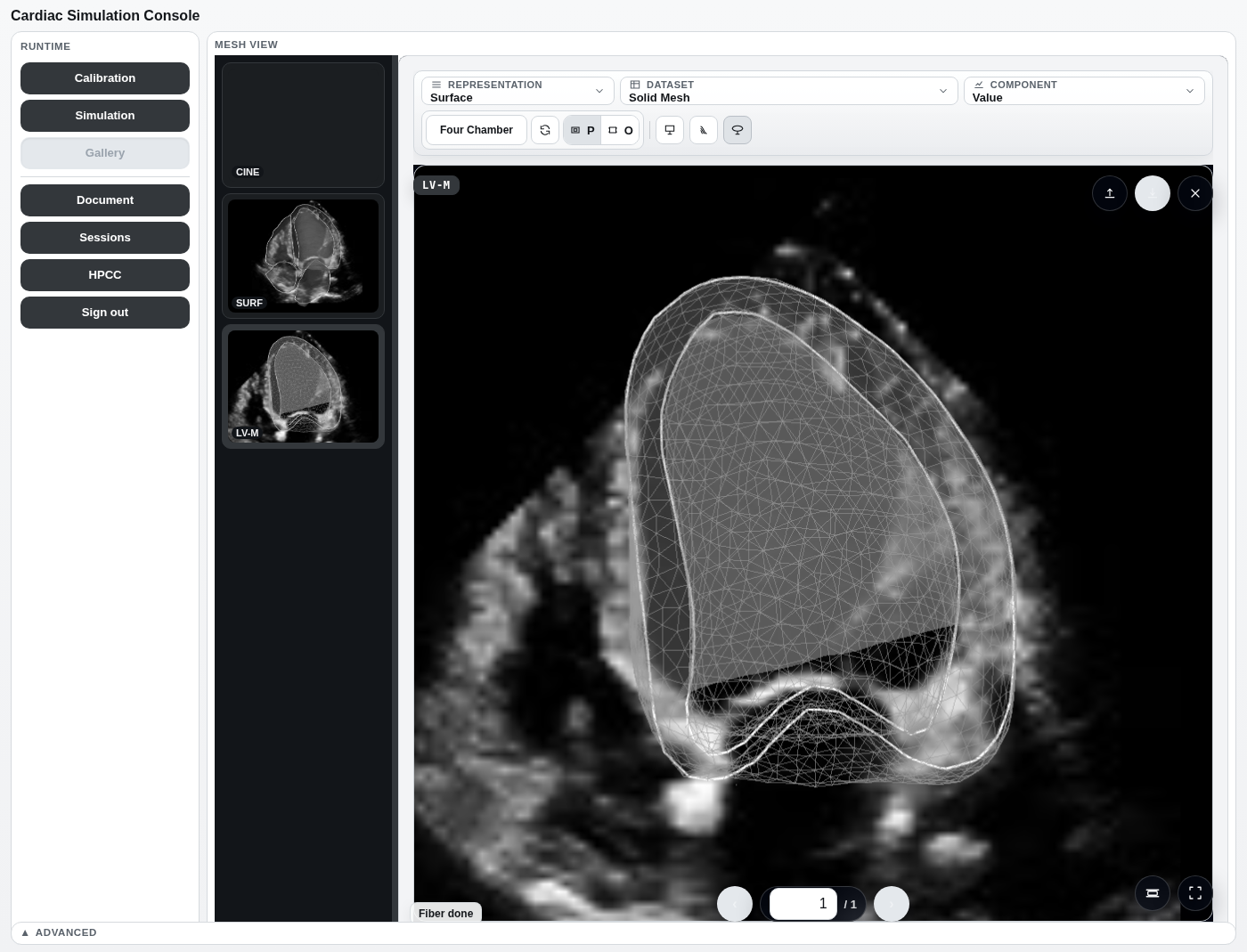
Sign in, and the console gives you two working surfaces. Mesh View, on the right, is where objects live: you drop files onto it, look at them in 3-D, and step between them. Runtime, the sidebar on the left, is where you act on the object you are looking at. Everything in this part of the guide happens in Mesh View.
There is exactly one place to look for progress, warnings, and failures: the status box at the top of the window. Whatever the platform is doing, it says so there. The Advanced drawer at the bottom holds the numeric progress bar and the raw, verbatim log for when a one-line message is not enough.
2. Choosing your input
Three kinds of thing can become a heart mesh. You do not have to tell the platform which one you are giving it — it recognises the file and takes the matching path.
| If you have | Bring | The platform will |
|---|---|---|
| A finished heart mesh | .xdmf together with its .h5, or a .zip of both |
Load it and show it straight away |
| A mesh from the solver's own format | a single self-contained .h5 |
Load it with whatever surface labels and fibers it already carries |
| An ultrasound cine | .avi |
Reconstruct the ventricle surface frame by frame, then build the mesh when you ask |
| A clinical echo study | one DICOM object, four-chamber view | Read the study's true physical scale, reconstruct, and build the mesh unprompted |
3. Path A — bringing your own mesh
Drag the file onto the viewer, or press Upload Object in the Mesh View
toolbar. A paired .xdmf must arrive together with the .h5 it names —
drop both, or zip them. Anything else is refused before it is stored, so an unusable object
never enters your workspace.
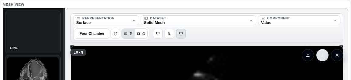
The mesh appears immediately, and the toolbar fills with what it found inside: the datasets it carries, and any vector fields you can display. Use Representation to switch between surface, wireframe, and points.
Where you go next depends on what the file already contains. A mesh exported from the solver usually arrives complete — surfaces already labelled, fibers already present — and is ready to simulate as-is. A bare geometry is not: run Infer LV facet regions and then Generate fiber fields from the toolbar, the same two operations that close out every other path (step 6).
4. Path B — an .avi echocardiogram
Drop the cine on the viewer. Two things happen at once: the movie becomes playable in the viewport straight away, and a reconstruction begins in the background. Reconstruction reads the ventricle out of the moving image and returns a surface for every frame of the cardiac cycle.
From those surfaces the platform picks the two frames that matter, by cavity size: end-diastole is the frame whose cavity is largest, end-systole the frame whose cavity is smallest. End-diastole is the configuration your mesh is built from, because it is the one the solver treats as the loaded reference state.
One caveat governs this path. An .avi carries no physical scale.
Nothing in the file says how many centimetres a pixel spans, so the reconstruction stays in
nominal units. Shape is faithful; absolute volumes are not. Use this path for geometry,
method development, and comparison between frames — not for a clinical volume. If you need
true dimensions, bring the DICOM instead.
When reconstruction finishes, the LV mesh builds automatically through the chain in step 6 — there is no button to press.
5. Path C — a DICOM echo study
Drop one four-chamber DICOM object. This path differs from the .avi in one
decisive respect and one convenient one.
The scale is real. A DICOM echo object states its own physical calibration — how much distance each pixel covers — and the platform reads it from the file. Every reconstructed surface is rescaled into physical units before anything is built from it, so the resulting mesh has true dimensions and its volumes mean what they say. If an object arrives without a usable calibration, the upload is rejected on the spot. The platform will not guess a scale, because a silently mis-scaled mesh is worse than no mesh.
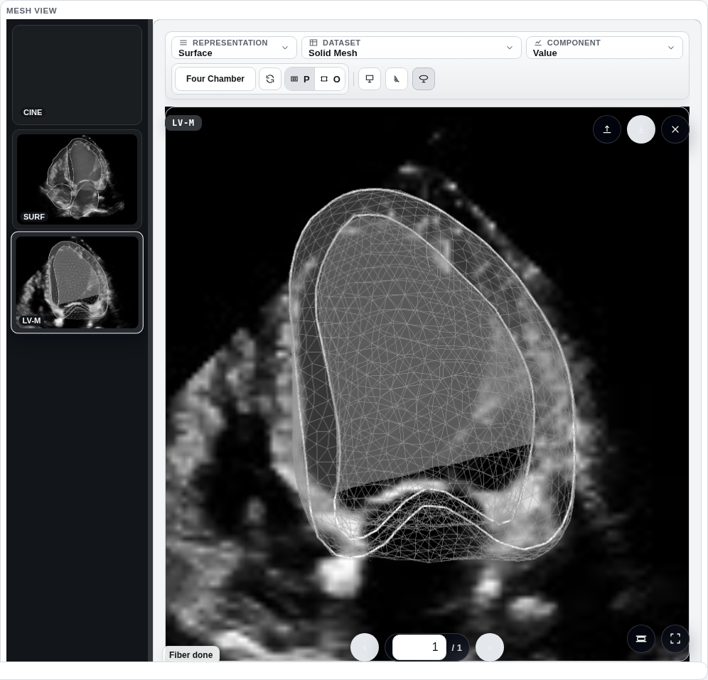
The mesh builds itself. There is no button to press. The object is decoded
into a viewable echo cine, reconstructed, rescaled, and carried through the whole build chain
automatically. When it settles you have three snapshots in the album, and you step between
them with the ‹ n / N › control beneath the viewport.
6. The shared build chain
Once a reconstruction exists, the .avi and DICOM paths are the same path. Six
steps run in order; the status box names each one as it starts.
- Volume. The ventricular wall — the shell between the inner and outer surfaces — is filled with tetrahedra. Mesh generation is not deterministic, so a result that misses the quality bar is thrown away and the step is retried, silently, until one passes.
- Trim. The cap at the base of the ventricle is cut away. What remains is the truncated chamber the solver expects: open at the base, closed at the apex.
- Adjust. The freshly cut mesh is re-meshed so element size and quality stay even across the new basal face rather than degrading where the knife went in.
- Adopt. The trimmed volume is promoted to a first-class mesh object. This is where the three input paths become one. From here nothing distinguishes a mesh reconstructed from a patient's echo from one you uploaded yourself.
- Facets. Every face on the boundary is classified as endocardium (the inner chamber wall), epicardium (the outer wall), or base (the flat annulus left by the trim).
- Fibers. Muscle direction is assigned throughout: a fiber direction, a sheet direction, and the sheet-normal perpendicular to both, rotating smoothly through the wall from the inner surface to the outer one.
The last two steps are exactly the two you can invoke by hand on an uploaded mesh. That is what makes the three paths one path: however the geometry arrived, it earns the same labels and the same fibers by the same means.
7. What “FE-ready” means
A mesh is ready for the finite-element solver when four things are true of it. The build chain exists to make all four true at once.
It is truncated
The basal cap is gone, leaving an open chamber with a clean rim.
Its boundaries are named
Endocardium, epicardium and base, so pressure can be applied inside and the base restrained.
It carries fibers
A fiber, sheet and sheet-normal direction everywhere, because myocardium does not pull equally in all directions.
Its elements are sound
Well-shaped tetrahedra, evenly graded, over a chamber whose topology is anatomically possible.
The fourth is the one the platform enforces on your behalf. Every candidate mesh is measured against a fixed set of hard requirements. No inverted or degenerate elements, no abrupt size jumps between neighbours, and exactly the surfaces a hollow ventricle should have. It must also show a single apex, a real cavity, and a basal ring that closes. A mesh that violates any one of them is rejected and rebuilt, never quietly accepted.
A much broader set of quality measures is recorded alongside every build without blocking it. That distinction is deliberate: a mesh is refused only when it would actually break the solve, not for being less than perfect. So a build fails for good in only two circumstances. Either the rebuilds were exhausted without a mesh that clears the hard requirements, or facet inference could not separate the wall into an inside, an outside, and a base. Both are reported, in words, in the status box.
8. Three common sessions
- “I have a patient's DICOM.” Drop it. Wait. Three snapshots appear — the echo, the end-diastolic surface, the mesh. The mesh has true dimensions. Nothing was pressed.
-
“I have an
.avi.” Drop it, watch the cine play while the reconstruction runs, then follow the six stages in the status box as the LV mesh builds automatically. Remember the geometry is in nominal units. - “I have a mesh from elsewhere.” Drop it and look at it. If it already has labelled surfaces and fibers, you are done. If not, run Infer LV facet regions, then Generate fiber fields.
9. When something goes wrong
The status box carries the reason; the raw log inside Advanced carries the detail. Nearly everything that stops a mesh from being built is one of these.
| What you see | What it means | What to do |
|---|---|---|
| The upload is refused before anything appears | An .xdmf arrived without the .h5 it names, or the two do not agree |
Drop both files together, or zip them and drop the zip |
| A DICOM is rejected on upload | The object states no usable physical calibration | Export the study again with its region calibration intact; the platform will not assume a scale |
| Reconstruction finishes with nothing to show | The ventricle could not be found in the images | Check the cine really is a four-chamber view, and that the ventricle stays in frame |
| The build retries, then gives up | No candidate mesh cleared the hard quality requirements | The reconstructed surface is usually the culprit — a self-crossing or a collapsed wall. Try a different frame or a cleaner acquisition |
| Facet inference fails | The wall could not be separated into inside, outside and base | Almost always an upstream geometry problem: inspect the trimmed mesh before rebuilding |
10. Mesh View keyboard shortcuts
While a mesh is loaded in the viewport, these keys and modified clicks drive facet selection, the brush, the reconstruction overlay, and undo.
| Action | Keys |
|---|---|
| Select a facet | Click |
| Add a facet to the selection | Shift + click |
| Remove a facet from the selection | Ctrl/Cmd + click |
| Assign a facet | Alt/Option + click |
| Toggle the brush | B |
| Change the brush size | + / - |
| Toggle the undeformed reference mesh | D |
| Show or hide the optional reference dataset | O |
| Cycle the echo image and its contours | E |
| Toggle the 2D echo-plane view | P |
| Undo | Ctrl/Cmd+Z |
| Redo | Ctrl/Cmd+Shift+Z |
| Close menus, clear the selection | Esc |
With an FE-ready mesh in hand, the rest of the platform opens up: establish its resting state, fit it to your measurements, and run a full cardiac cycle. That is Part II.